Lộc Lương

In retrospect, I recall that my math professor at my Vietnamese college introduced me “neural network” around late 2016 or early 2017. I’m pretty sure that at that time I didn’t know any thing about artificial neural network (ANN), or machine learning (ML), or deep learning (DL). I got a stack of papers printed out to read some introduction about ANN, and I was so excited that I wish I’d been introduced to it sooner. I spent a few days and nights (maybe even more I couldn’t remember) just to get a good understanding behind it, including the maths (e.g., algebra, optimization) and codes. It is interesting that ANN is able to approximate any continuous, smooth function if it has enough neurons. And this is already rigorously proved as the universal approximation theorem.

When I did my Master in petroleum at New Mexico Tech, I started to accumulate formal language of optimization methods, and I was wondering if I could do a pet project combining neural nets with a global optimization algorithm to solve the inverse problem.

History matching (or formally known as inverse problem) is one of the most important problem in reservoir engineering. Technically, in forward problem we apply a simulator (or a black box) to model a physical system of interest: parameters ($\theta$) $\rightarrow$ model $\rightarrow$ output (simulated data). In contrast, we do the backward for the inverse problem, we compared real-world observation data with simulated data to figure out a set of parameters that best represents underlying physical model: data (observations) $\rightarrow$ model $\rightarrow$ parameters ($\theta$). In the context of petroleum engineering, this is defined as the process of finding an appropriate set of parameters which can reasonably (ideally best) reproduce the dynamical behavior of a reservoir system (multiphase flow of oil, gas, and water).

Inverse problem is often an ill-posed problem, meaning that there is no unique solution to the problem. Strictly speaking, in a well-pose problem, there needs to be a solution, and the solution need to be unique, as well as stable. Fail of any one of these three conditions, we can call the problem ill-posed. In practice, instability often manifests as numerical ill-conditioning where a small perturbation or err in the input can produce a large errors in the outcome.

On the other hand, simulating a multiphase flow problem is often computationally expensive. Even in some cases, engineers prefer simpler analytical methods, such as decline curve analysis or material balance, to study reservoir behavior or estimate reserve. Due to the complexity and computational overhead of simulation runs, we’d want alternative approaches. One such approach is to couple a neural networks and particle swarm optimization to solve the history matching problem.

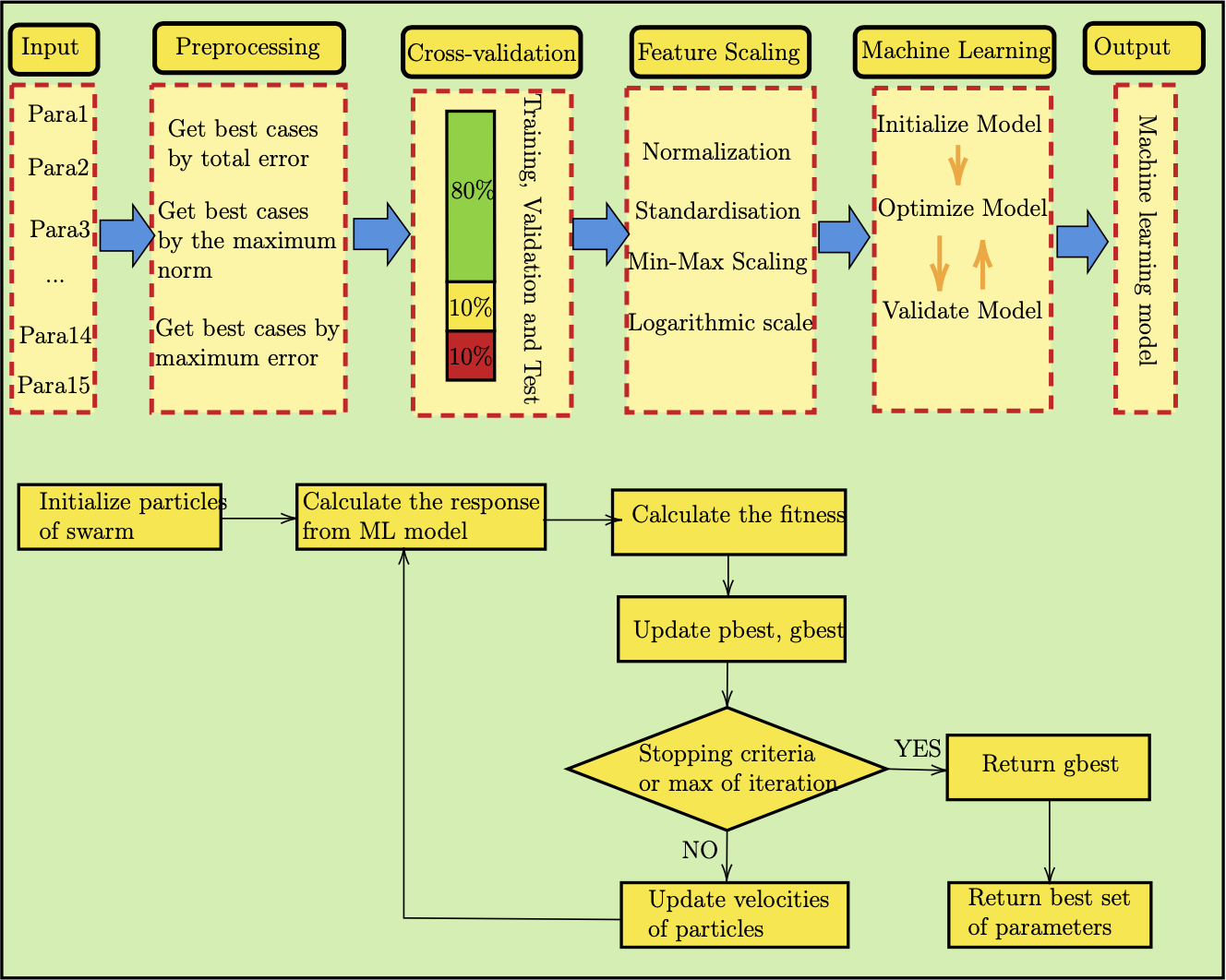
To design a machine learning model (specifically a neural net) to perform the history matching of a black oil reservoir (oil, gas, water), we need to have a set of simulation output based on varying model parameters. A bit of information on the reservoir: it has been producing for 50 years; historical data contains all information of dynamical simulation and production. There were a total of 187 simulation runs with certain output, and a set of 15 reservoir properties (e.g., average porosity, permeability, bottom hole pressure (BHP), temperature).

Overview of a neural network

In a typical multi-layer neural networks, beside the input and output layers, there are several hidden layers in the middle. Figure above is an example of fully connect multi-layer neural network with three hidden layers. Let denote the output of each unit as $a$, therefore the output of a layer $(l)$ is $\mathbf{a}^{(l)}$. In a neural network of $L$ layers, there are corresponding $L$ matrices of coefficients ($\mathbf{W}^{(l)} \in \mathbb{R}^{d^{(l)}\times d^{(l+1)}}$) that represent connection between layer $l-1$ and layer $l$. Note that layer $0$ is the input layers. Bias of layer $l$ is usually denoted by $\mathbf{b}^{(l)} \in \mathbb{R}^{d^{(l)}}$. We then can define $\mathbf{\theta}^{(l)} = [\mathbf{b}^{(l)}, \mathbf{W}^{(l)}]$ as the weight matrix of layer $(l)$. The output from each layer can be written as:

$$ \mathbf{a}^{(l)} = f(\mathbf{W}^{(l)}\mathbf{a}^{(l-1)} + \mathbf{b}^{(l)}) = f(\mathbf{\theta}^{(l)}\mathbf{a}_{\ast}^{(l-1)}) $$

where $\mathbf{a}_{\ast}^{(l-1)}$ is the concatenate form of a column vector of $1$ and $\mathbf{a}^{(l-1)}$.

Now, we can define the loss function between the output or model response and actual data or observations. In a regression probelem, mean square error (MSE) function is often used because it is a convex function as well as for easier calculation of derivatives. That means we can apply gradient-based optimization techniques. The loss function is defined as:

$$ J(\mathbf{W}, \mathbf{b}) = \frac{1}{N}\sum_{i=1}^{N}||{y_i - \hat{y}_i}||_2^{2} $$

where $\mathbf{W}, \mathbf{b}$ are two sets of all weight matrices $\mathbf{W}^{l}$ and biases $\mathbf{b}^{l}$, $y_i$ is model output from neural network and $\hat{y}_i$ is actual data. Or:

$$ J(\mathbf{\theta}) = \frac{1}{N}\sum_{i=1}^{N}||{y_i - \hat{y}_i}||_2^{2} $$

As I don’t use gradient descent for the optimizer, I’m just giving a few lines about this algorithm here. In training neural networks or machine learning models, gradient descent (GD) and its variants are by far the most popular techniques. Gradient descent is an algorithm used to optimize the objective function $J(\mathbf{\theta})$, with respect to the parameter $\mathbf{\theta} \in \mathbb{R}^d$, by gradually updating the parameter $\mathbf{\theta}$ in the opposite direction to the gradient of the objective function. The learning rate $\eta$ determines the size of each backward jump of $\mathbf{\theta}$. The advantages of GD are the ease of implementation and low memory cost, while the drawback is the convergence time or local minima. In machine learning or deep learning area, we use this algorithm to update model weights $\mathbf{\theta}$. The general definition of gradient descent algorithm is followed by:

$$ \mathbf{\theta} = \mathbf{\theta} - \eta\nabla J(\mathbf{\theta}) $$

Particle Swarm Optimization (PSO)

PSO is a nature-inspired stochastic optimization algorithm that mimic the flocking of birds, or movement of school of fish. The idea behind this algorithm is that particles will communicate the information they find with others, and update their velocity based on the local best (pbest) and global best particle (gbest). The swarm will update best result as when the new global best is found, and each particle tend to move toward the personal best and global best. PSO is a global optimizer which aims to find global minima or maxima of an objective function. Here is the general updating rule for the PSO algorithm:

PSO

Hyperparameters:

• ( w ): inertia weight (typically slightly less than 1)
  
• ( c_1 ): cognitive coefficient — influence of personal best
  
• ( c_2 ): social coefficient — influence of global best
  
• ( r_1, r_2 ): random values in ([0,1]), introducing stochasticity

Below is a pseudo code in Python:

# PSO Algorithm
initialize particles (x_i, v_i) randomly
for t in range(max_iter):
    for each particle i:
        evaluate fitness f(x_i)
        if f(x_i) < f(pbest_i): pbest_i = x_i
        if f(x_i) < f(gbest):   gbest   = x_i
    for each particle i:
        v_i = w*v_i + c1*r1*(pbest_i - x_i) + c2*r2*(gbest - x_i)
        x_i = x_i + v_i
return gbest

How to train a machine learning model

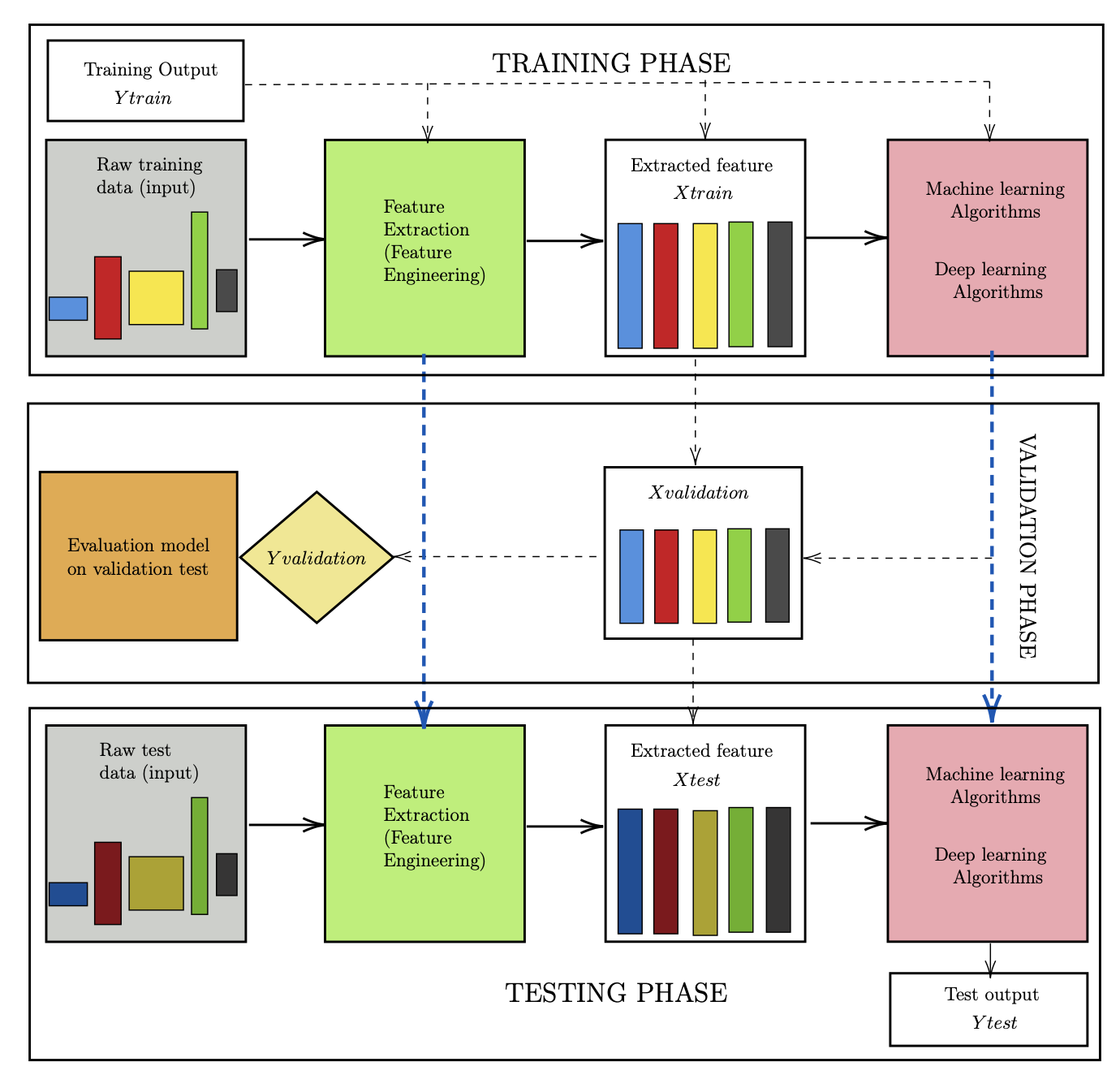
There are three phases in this process: training, validation, and testing. In the training phase, we need to design two blocks (green and pink), which are the feature extractor and the main algorithm. The input data represents all available information about the system. For example, for an image, it is the value of each pixel; for audio, it is the signal. In this project, the raw input may include all reservoir information such as permeability, porosity, relative permeability, bottom-hole pressure, initial state, etc.

However, the raw data is usually not in vector form, does not have the same dimensions, and often contains noise. Missing values may also be encountered. Therefore, a feature extraction step is required to transform the raw data into a clean, structured, and informative representation. The extracted features are then used as inputs to train the machine learning or deep learning model.

In the learning algorithm stage, the extracted features, along with (optionally) labeled outputs, are used to construct a model that captures the relationship between inputs and outputs. An important point is that when building the feature extractor and the main algorithm, we should not use any information from the test dataset. The test data must be treated as completely unseen during training.

In the testing phase, for new raw input, we use the feature extractor created above to generate the corresponding testing feature vectors. These features are then fed into the trained model to produce predictions. The performance of the model is evaluated by comparing these predictions with the true outputs.

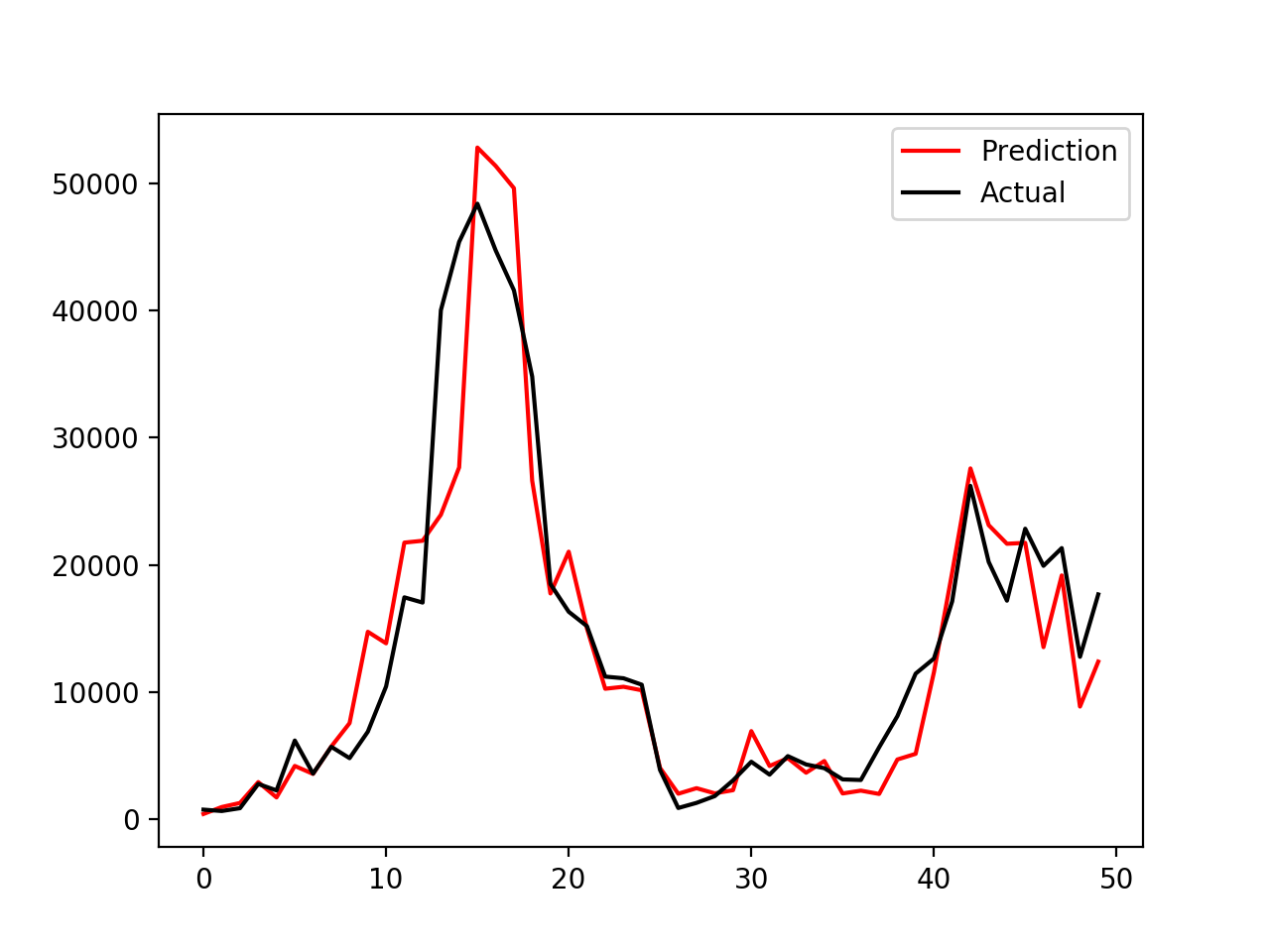
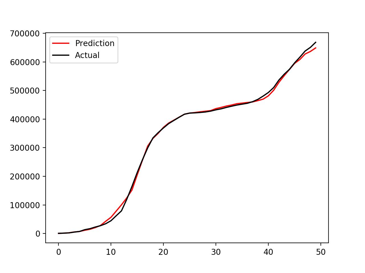
Some interesting results

The left panel shows the time series of oil production, while the right panel shows the cumulative oil production. This coupled model (PSO–NN) does a reasonably good job at matching the observed data. In this work, I only used a simple multilayer fully connected neural network coupled with PSO for optimization. More advanced models, such as Restricted Boltzmann Machines (RBM), Long Short-Term Memory networks (LSTM), or deeper neural networks, can also be used to improve the surrogate modeling. In addition, other optimization algorithms, such as genetic algorithms (GA), could be combined with these models to further enhance performance and robustness

You can see this GitHub repository for results and implementation details.